Artificial neural networks such as MLP (Multilayer Perceptron) and CNN (Convolutional Neural Network) have been successfully used to statically classify malware (Raff et al. 2017; Vinayakumar and Soman 2018; Krčál et al. 2018). This post should help beginners in deep learning to apply these models in practice as we walk through a task of static malware classification. We assume that the reader has just explored what MLP and CNN are but hasn’t used them yet. We will not focus on the code but rather guide the reader through the overall process and hopefully provide useful intuition along the way. We will also explain various metrics that are useful in binary classification.
Data Set
The EMBER data set (Anderson and Roth 2018) contains features extracted from executable files in the PE (Portable Executable) format. Each file is abstracted into a JSON object which can be subsequently transformed into a feature vector containing 2351 dimensions. Besides the JSON data, the authors of the data set also provided methods for transforming it into the feature vectors. These methods implement embedding techniques such as the hashing trick where appropriate. We focus on EMBER 2018, which contains:
- Training data:
- 200,000 unlabelled samples,
- 300,000 malicious samples,
- 300,000 benign samples.
- Test data:
- 100,000 malicious samples,
- 100,000 benign samples.
Data Preprocessing
At the very beginning, the unlabelled samples were removed. The first obstacle that emerged during the process of building our classifiers was that it was not possible to train them on the raw 2351-dimensional vectors provided by the data set. The accuracy even on the training data was always no better than that of a random classifier, regardless of the architecture of the network. On the other hand, the accuracy of the gradient boosted decision tree provided by the authors of the data set was 93.61%. The reason the neural networks failed was that the variance of the data was too high, namely \(8.82 \times 10^{14}\)8.82 10 14. We decided to standardize the data by calculating the standard score. Since the resulting data contained NaN (Not a Number) values, the accuracy was still no better than random. After setting the NaN values to zero, the neural networks started learning.
The next step was to examine the data by performing a PCA (Principal Component Analysis). The PCA revealed that the first dimension of the new space contains approximately 3.5% of variance and that the first 1024 components contain approximately 90% of variance. Since training with 1024-dimensional vectors is much faster than training with the original vectors, and the loss of information was acceptable, we decided to utilize this reduction.
Experiments
The neural networks in the experiments are implemented using the Keras library. We also employed a hyper-parameter optimization technique called random search, implemented in the Keras Tuner library.
Besides the accuracy metric for model evaluation, we also consider the precision and recall metrics. These metrics use the notion of true and false positives and negatives. In malware detection, a false positive means that a file is considered malicious even though it is actually harmless. On the other hand, a false negative means that a malicious file has not been detected.
In our case, precision describes the cost of false positives (when our model falsely determines that a benign file is malicious) and is defined as follows:
\[ \text{Precision} = \frac{\sum \text{True Positive}}{\sum \text{True Positive} + \sum \text{False Positive}}. \]
Recall is defined in a similar fashion:
\[ \text{Recall} = \frac{\sum \text{True Positive}}{\sum \text{True Positive} + \sum \text{False Negative}}. \]
Note that the denominator in the definition of recall is in fact the sum of all actually positive samples. Recall describes how good our model is at capturing files that are truly malicious and as such can be seen as the probability of detection.
We also use the terms FPR (False Positive Rate) and TPR (True Positive Rate). FPR is defined as follows:
\[ \text{FPR} = \frac{\sum \text{False Positive}}{\sum \text{True Negative} + \sum \text{False Positive}}. \]
Notice again that the denominator is the sum of all truly negative samples. TPR is defined in the same way as recall and is therefore just a synonym. We utilize ROC (Receiver Operating Characteristic) curves that show the relation between FPR and TPR. The goal for a binary classifier is to have high TPR at low FPR. We can therefore compare our models based on this metric. Another metric is the AUC (Area Under the Curve). This metric represents the area under the ROC curve. An ideal classifier would have an AUC of 1.
Multilayer Perceptron
Since machine learning utilizing neural networks is an empirical realm, we start by experimenting with the network architecture and its hyper-parameters. In order to estimate these parameters, the model was run multiple times on a reduced data set for 5 epochs.
The MLP model was run 6000 times by the random search routine with various hyper-parameters, and the best 10 runs had the following common properties: dropout was set to zero, the activation function was ReLU (Rectified Linear Unit), and the optimizing method was Adam (Adaptive Moment Estimation). The layer width of the best-performing models was mostly between 64 and 512 neurons. Larger or smaller layers were not preferred. These results provided an elementary insight into suitable models, and the preceding hyper-parameters were set for all subsequent models.
The next step was to estimate the most appropriate depth of the network. The model was run again 3000 times, and the best-performing network had 4 layers with 512 neurons, 2 layers with 128 neurons, and one layer with 64 neurons. This network was then retrained on the full data set for 50 epochs, as further training did not provide any performance improvement.
The last layer always had one neuron with a sigmoid activation function. The loss function was binary cross-entropy. The learning rate was chosen automatically by the Keras library.
Convolutional Neural Networks
As mentioned in the introduction, CNNs have also been used to statically analyze malware. We built a 1D CNN in a similar fashion to that described in the previous section. This time, however, the search for hyper-parameters was much slower due to higher computational demands — the model was much slower to train and the hyper-parameter search space was much larger. The model was run 3000 times, and the best-performing network had three convolutional layers with 16 kernels, each of size 32. There were also four dense MLP layers with sizes 512, 256, 128, and
- The stride parameter of the convolutional layers was set manually to two in
order to speed up training. The rest of the hyper-parameters were kept the same as in the MLP model.
Researchers have also tried to detect malicious software by transforming it into images and then applying 2D CNNs (Kabanga and Kim 2018; Kalash et al. 2018). We also tried such an approach: we transformed the feature vectors into matrices (with 32 rows and columns, since the feature vectors have 1024 dimensions) and then naively tried to adapt and retrain a pre-built CNN called VGG16 (Simonyan and Zisserman 2014). The motivation was to find out whether a network with an architecture that works well for recognizing general images could also perform well in our domain. Originally, the network had 1000 output neurons. We added one more neuron on top of this layer in order to transform the network into a binary classifier. The activation function of this neuron was a sigmoid function. The optimizing method and loss function were also chosen to be the same as in the MLP model. The convolutional networks were also trained on the full data set for 50 epochs.
Results
Table bk. Metrics comparison.
| Accuracy [%] | Precision [%] | Recall [%] | |
|---|---|---|---|
| MLP | 95.04 | 95.52 | 94.51 |
| GBDT | 93.61 | 92.40 | 95.05 |
| CONV | 93.51 | 93.22 | 93.85 |
| Adapted VGG16 | 93.13 | 93.94 | 92.22 |
| MLP (no preproc.) | 52.73 | 51.41 | 99.59 |
Table bk shows the metrics comparison of the trained models on the test data. The MLP model has the highest accuracy and also outperforms the baseline GBDT provided by the EMBER library. It is also worth noting that the MLP model has a much simpler architecture than the VGG16 network, for example.
Figure bm. ROC comparison.
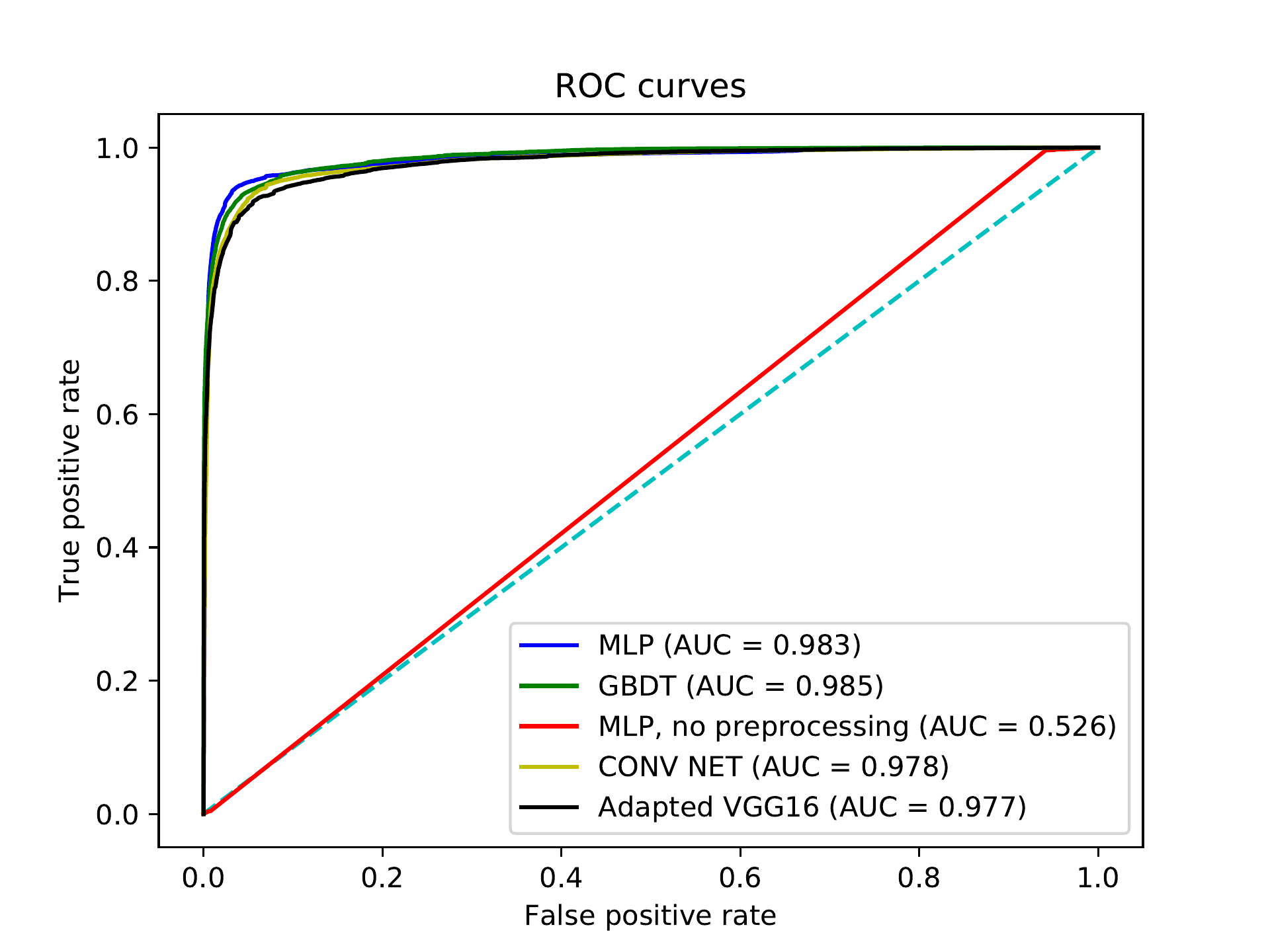
Figure bc. ROC comparison (zoomed-in).
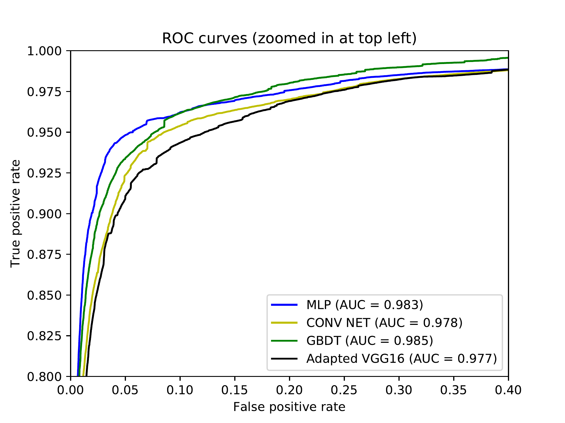
Figures bm and bc show the ROC curves for our trained models. The MLP model has the best ROC up to around 15% FPR, where it is surpassed by the GBDT model. The adapted VGG16 actually has the poorest performance.
Figure bp. MLP classification distribution.
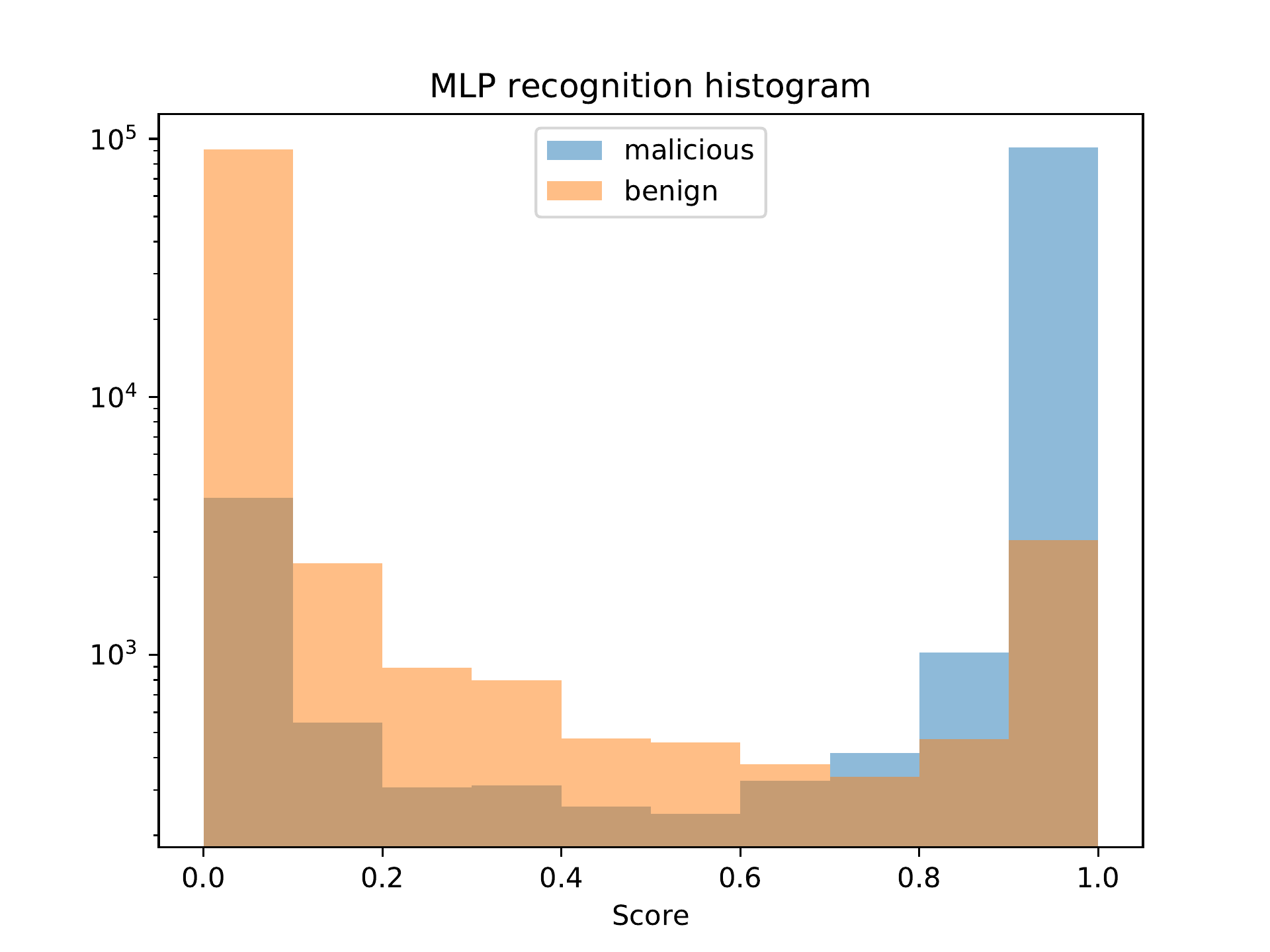
Figure bp depicts the classification distribution of the MLP model. We can see that for most samples, the model gives a confident correct answer. However, there is also a considerable number of samples for which the model gives the wrong answer with certainty as well.
Figure bq. CONV classification distribution.
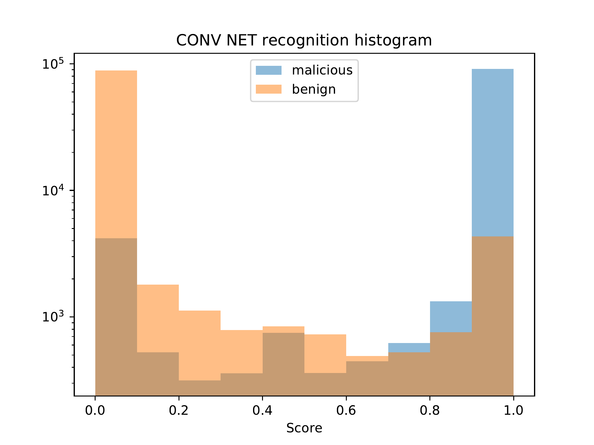
Figure bx. Adapted VGG16 classification distribution.
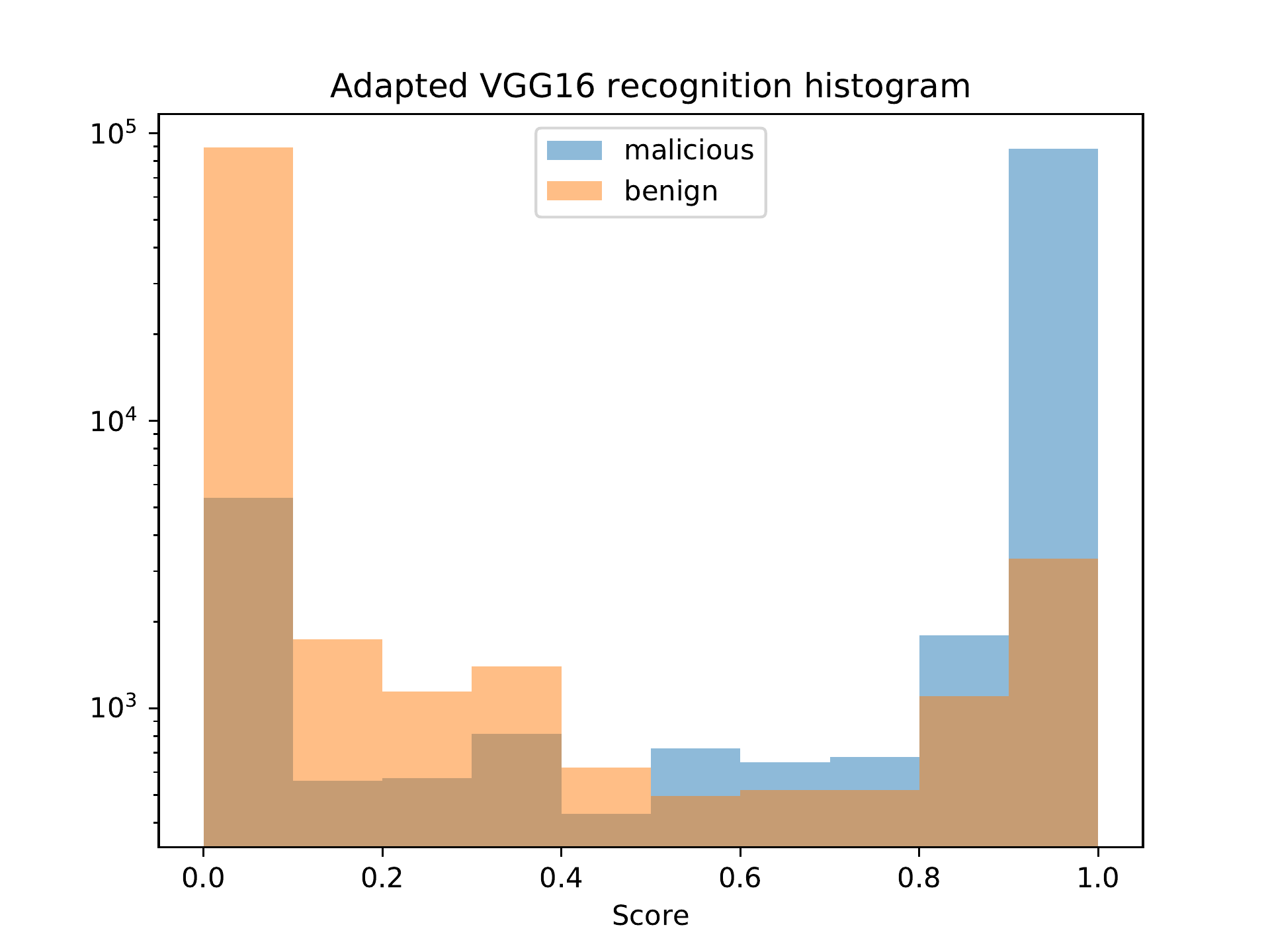
Figures bq and bx show that the convolutional networks have similar behavior to the MLP model with regard to the classification distribution.
Figure bo. MLP (no preprocessing) classification distribution.
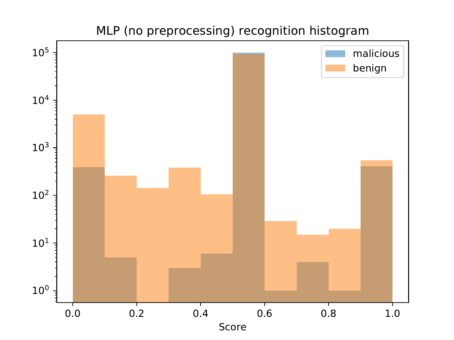
Figure bo shows the classification distribution for the MLP model which classified the raw data from the data set. We can see that the model classified most samples as positive (the output value for most samples was 0.5). This is the reason why this model has the highest recall in Table bk. However, the precision is very low, and since the data set contains an equal number of benign and malicious samples, the accuracy is close to that of a random classifier, which is exactly 50%.
Dimensionality Reduction Experiments
Besides PCA, a VAE (Variational Autoencoder) can also be used to reduce the dimensionality of the data. We experimentally built and trained a VAE that reduces our data to three dimensions. The architecture and hyper-parameters of the encoder and decoder of the VAE were chosen to match the best-performing MLP model.
Figure bt. Dimensionality reduction by a VAE.
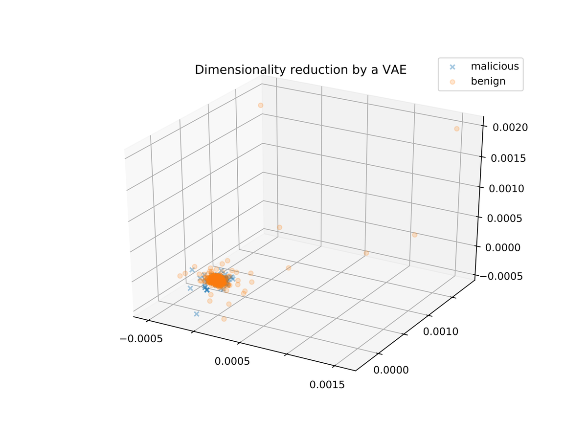
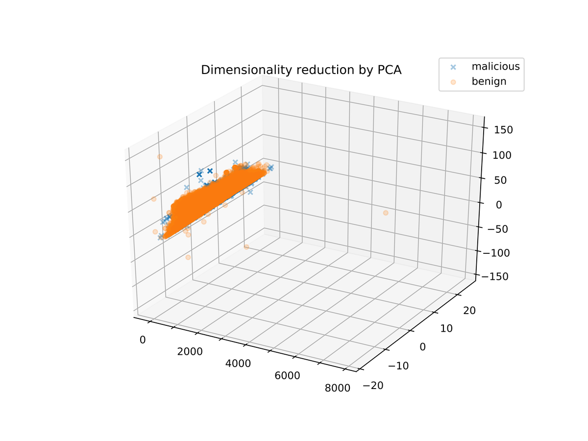
Figure bt shows the resulting three-dimensional data. We see that all the samples are gathered in a single dense cloud, which means that the classification is not a straightforward task. For comparison, Figure b1 shows the same data after a reduction to three dimensions by PCA.
Figure b1. Dimensionality reduction by PCA.