I feel I am nibbling on the edges of this world when I am capable of getting what Picasso means when he says to me — perfectly straight-facedly — later of the enormous new mechanical brains or calculating machines: “But they are useless. They can only give you answers.” — William Fifield, Pablo Picasso: A Composite Interview, The Paris Review 32
The principle of algebraic cryptanalysis consists in transferring the problem of breaking a cryptosystem to the problem of solving a system of multivariate polynomial equations over a finite field. The process is divided into two steps. The first step uses the cipher’s structure and supplemental information to create a system of equations that describes the behavior of the cipher for a specific case. Several papers (Cid, Murphy, and Robshaw 2005; Bulygin and Brickenstein 2010) present approaches for constructing polynomial equations for AES. The second step involves solving the polynomial system to derive the secret key. While the method for deriving the system depends on the cipher, the method for solving the system may be independent of it.
In a companion post on equation systems, we model the small scale variants of AES as systems of polynomial equations over \(\mathrm{GF}(2)\)GF(2) that involve only the variables of the initial key. In this post, we attempt to solve such systems using Gröbner bases (specifically the F4 algorithm (Faugère 1999)) and compare the results to a SAT solver. We present some reduction techniques for reducing the computational complexity of solving the polynomial systems and provide an insight into the propagation of diffusion within the cipher. For example, one of the attacks can recover the secret key for one round of AES-128 in under a minute, requiring only two known plaintext–ciphertext pairs.
The experiments were carried out on GNU/Linux 5.4 running on two Intel Xeon Gold 6136 processors with 768 GB DDR4 memory evenly split into 12 modules. The baseboard was Supermicro X11DPi-NT. The initial polynomial systems containing auxiliary variables were generated using Martin Albrecht’s implementation of the small scale variants of AES in SageMath 9.1 (The Sage Developers 2020), which also uses Python 3.7.3 and PolyBoRi (Brickenstein and Dreyer 2009). The systems were solved in Magma V2.25-5 (Bosma, Cannon, and Playoust 1997) and CryptoMiniSat (Soos, Nohl, and Castelluccia 2009). The source code for the experiments can be found at https://github.com/upbqdn/yaac. The generation and preprocessing of the polynomial systems was parallelized across all 24 available cores. Magma, however, could only solve one system on a single core, so to keep the comparison fair, we explicitly restricted CryptoMiniSat to one core as well.
As stated in Definition fg, we may regard a system of polynomials as a basis of an ideal \(I\)I. We can then compute the reduced Gröbner basis of \(I\)I under the lexicographic order, and by applying the Elimination Theorem, we can easily obtain the solution. We have demonstrated the use of this theorem in Example db and Example di, and as we have discussed in AES as a System of Equations, the solution represents the secret key.
Systems with Auxiliary Variables
Table ri shows the results of initial experiments with systems of equations containing auxiliary variables. We generated the systems in SageMath for various versions of \(\mathrm{SR}(n, r, c, e)\)SR(n, r, c, e), and we subsequently attempted to solve these systems by the F4 algorithm implemented in Magma and by CryptoMiniSat.
Since we work over \(\mathrm{GF}(2)\)GF(2), the polynomials can be viewed as logical formulas in algebraic normal form (ANF). SageMath supports a conversion from ANF to CNF (conjunctive normal form). Formulas in CNF can be passed to CryptoMiniSat and the initial key can then be easily recovered from the solution. We have included the SAT solver so that we can compare it to the performance of the F4 algorithm, and we can see in the table that the solver performs much better. The SAT solver also takes a negligible amount of memory, so this value is not stated in the table.
The average number of monomials per polynomial is between 6 and 8 when \(e = 4\)e = 4 and between 18 and 20 when \(e = 8\)e = 8. Both the average and highest degrees of monomials are equal to two, so all polynomials are quadratic or linear. In our experiments, we do not consider the ciphers with \(r < 2\)r < 2 or \(c < 2\)c < 2 as these have the matrices for MixColumns and ShiftRows reduced to \((1)\)(1). Recall that the dimensions of the state array \(r\)r and \(c\)c are restricted to the values 1, 2, and 4; the exponent \(e\)e can be either 4 or 8; and for the number of rounds \(n\)n, we have \(1 \le n \le 10\)1 n 10.
The column named Vars contains the number of variables in the whole polynomial system and the column named Polys contains the number of polynomials in the system. We measured the runtime and memory consumption only during the solving of the polynomials since the preparation of the system takes only a fraction of the resources relative to solving it.
Recall that the key size for \(\mathrm{SR}(n, r, c, e)\)SR(n, r, c, e) is given by the product \(rce\)rce. Notice that we were not able to compute the solution for even one round of \(\mathrm{SR}(n, 4, 4, 8)\)SR(n, 4, 4, 8), the key size of which is 128 bits. On the other hand, the SAT solver could quickly compute the solution for all ten rounds of \(\mathrm{SR}(n, 2, 2, 4)\)SR(n, 2, 2, 4).
Table ri. Initial experiments with systems containing auxiliary variables.
| Cipher | Key bits | Vars | Polys | F4 Time | F4 Mem. | SAT Time |
|---|---|---|---|---|---|---|
| SR(1, 2, 2, 4) | 16 | 72 | 120 | 1 s | 33 MB | 2 s |
| SR(2, 2, 2, 4) | 16 | 128 | 224 | 19 s | 848 MB | 12 s |
| SR(3, 2, 2, 4) | 16 | 184 | 328 | 4 h | 76 GB | 17 s |
| SR(4, 2, 2, 4) | 16 | 240 | 432 | — | — | 27 s |
| SR(10, 2, 2, 4) | 16 | 576 | 1056 | — | — | 50 s |
| SR(1, 4, 2, 4) | 32 | 144 | 240 | 48 s | 981 MB | 9 s |
| SR(2, 4, 2, 4) | 32 | 256 | 448 | — | — | 1.5 min |
| SR(3, 4, 2, 4) | 32 | 368 | 656 | — | — | 63 h |
| SR(1, 2, 4, 4) | 32 | 136 | 216 | 3 s | 67 MB | 11 s |
| SR(2, 2, 4, 4) | 32 | 240 | 400 | — | — | 33 s |
| SR(3, 2, 4, 4) | 32 | 344 | 584 | — | — | 15.5 min |
| SR(4, 2, 4, 4) | 32 | 448 | 768 | — | — | 34 h |
| SR(1, 4, 4, 4) | 64 | 272 | 432 | — | — | 2.5 min |
| SR(1, 2, 2, 8) | 32 | 144 | 240 | 1 min | 2.2 GB | 22 s |
| SR(2, 2, 2, 8) | 32 | 256 | 448 | — | — | 11.5 min |
| SR(1, 4, 2, 8) | 64 | 288 | 480 | — | — | 41.5 min |
| SR(1, 2, 4, 8) | 64 | 272 | 432 | — | — | 4 min |
| SR(1, 4, 4, 8) | 128 | 544 | 864 | — | — | — |
Systems without Auxiliary Variables
Table rs contains the results of experiments with systems that contain only the variables of the initial secret key. We eliminated the auxiliary variables by a gradual substitution of the variables of the initial key through the system, starting by adding the known plaintext bits and ending by adding the known ciphertext bits. The time required for this substitution is stated in the column named PT. This system always contains \(k\)k polynomials in \(k\)k variables where \(k\)k is the number of key bits. Since \(k\)k is the number of variables and we work over \(\mathrm{GF}(2)\)GF(2), \(k\)k is also the maximal limit of the total degree of the polynomials.
All further experiments are carried out with systems of polynomials involving only the variables of the initial key. In systems with auxiliary variables, the structure of the polynomial systems derived from different plaintexts remains unchanged. Only the initial and final polynomials that add the bits of the plaintext and ciphertext differ by this bitwise addition. Since we have eliminated the auxiliary variables by a gradual substitution of the initial key bits starting from the initial plaintext addition, each of the \(k\)k polynomials now depends on the choice of plaintext and its corresponding ciphertext. Since the structure of each polynomial system is now different, the time and memory required for obtaining the solution started to differ as well, especially the time required by the SAT solver. For this reason, all the following tables contain average results of five different runs for each experiment. The results for the SAT solver still differ across tables for the same experiment, so even more than five runs would be needed for further investigation. Nevertheless, we restricted ourselves to this number due to limited time resources.
The column named AMP contains the average number of monomials per polynomial in the whole system. This number grows rapidly as \(n\)n increases. The maximal limit of the number of monomials in one polynomial is \(2^k - 1\)2 k - 1. When \(n = 1\)n = 1 and \(e = 4\)e = 4, the average degree of monomials is 2 and the highest degree is 3. When \(n = 2\)n = 2, the average and highest degrees are 5 and 9, respectively. Note that the average degree has its maximum at \(\frac{k}{2}\)k2. We were not able to generate systems with \(n > 2\)n > 2 and \(r, c > 2\)r, c > 2 for \(e = 4\)e = 4. For \(n = 1\)n = 1 and \(e = 8\)e = 8, the average degree is 4 and the maximal degree is 7. We were not able to generate systems with \(e = 8\)e = 8 and \(n > 1\)n > 1 (recall that we do not consider the cases when \(r < 2\)r < 2 or \(c < 2\)c < 2). The overall performance is worse compared to Table ri and the SAT solver still outperforms the F4 algorithm. Moreover, we were able to solve fewer systems than in the previous experiments.
Table rs. Experiments with systems with no auxiliary variables. PT is the preprocessing time required to obtain the system. AMP is the average number of monomials per polynomial.
| Cipher | Key bits | PT | AMP | F4 Time | F4 Mem. | SAT Time |
|---|---|---|---|---|---|---|
| SR(1, 2, 2, 4) | 16 | 1 s | 20 | 1 s | 33 MB | 1 s |
| SR(2, 2, 2, 4) | 16 | 1 s | 2475 | 2.5 min | 4.8 GB | 1 min |
| SR(3, 2, 2, 4) | 16 | 8 s | 32784 | 8.5 min | 18.5 GB | 13 min |
| SR(10, 2, 2, 4) | 16 | 2.5 min | 32814 | 9 min | 19.5 GB | 14 min |
| SR(1, 4, 2, 4) | 32 | 1 s | 37 | 55 s | 1.2 GB | 1 s |
| SR(1, 2, 4, 4) | 32 | 1 s | 23 | 13 s | 671 MB | 1 s |
| SR(1, 4, 4, 4) | 64 | 4 s | 40 | — | — | 2 min |
| SR(1, 2, 2, 8) | 32 | 8 s | 314 | — | — | 1.5 min |
| SR(1, 4, 2, 8) | 64 | 18 s | 567 | — | — | 33 min |
| SR(1, 2, 4, 8) | 64 | 14 s | 348 | — | — | 1.5 h |
Full Diffusion
In Table rs, the AMP value and the solving time and memory are almost the same for \(\mathrm{SR}(3, 2, 2, 4)\)SR(3, 2, 2, 4) and \(\mathrm{SR}(10, 2, 2, 4)\)SR(10, 2, 2, 4). This means that the maximal diffusion for \(\mathrm{SR}(n, 2, 2, 4)\)SR(n, 2, 2, 4) is reached in the third round of the cipher and the subsequent rounds do not provide any further security as regards the algebraic cryptanalysis, except for a longer time required for the generation of the polynomial system. This observation seems to be in line with the statements made in (Aumasson 2019). Table rz provides a deeper insight into the distribution of monomials in \(\mathrm{SR}(3, 2, 2, 4)\)SR(3, 2, 2, 4). At full diffusion, the expected number of monomials of degree \(d\)d should be equal to \(\frac{1}{2} \binom{k}{d}\)12 {k}{d} where \(k\)k is the number of variables. Since we have \(\mathrm{SR}(3, 2, 2, 4)\)SR(3, 2, 2, 4), we get \(k = 2 \cdot 2 \cdot 4 = 16\)k = 2 2 4 = 16 — recall that we also have \(k\)k polynomials in the whole system. In Table rz, the expected value is stated in the last row. All the polynomials follow this value very closely, meaning that it is not possible to get much closer to the expected value in the subsequent rounds. For this reason, we do not consider the rounds between the third and tenth one. The table also shows that the average monomial degree is 8 for each polynomial, which is half of the maximal degree, and that no polynomial significantly differs from the expected values for monomial degrees. The second last row shows the average value for all of the polynomials.
The last column contains the number of all monomials in the polynomial. At full diffusion, this number should be equal to \(\sum_{d=0}^{16} \frac{1}{2} \binom{k}{d} = \frac{2^{16}}{2} = 32768\), so that every polynomial contains half of all possible monomials. The number of monomials is close to the expected value for each of the polynomials as well. Considering the full diffusion again, each variable should appear in half of the monomials in every polynomial, so the expected frequency is \(\frac{2^{16}}{4} = 16384\)2 16{4} = 16384. In the actual system described in Table rz, the most frequent variable had 16446 occurrences and the least frequent variable had 16393 occurrences; these are aggregated values.
Table rz. Distribution of monomials of a given degree in \(\mathrm{SR}(3, 2, 2, 4)\)SR(3, 2, 2, 4).
| Poly | 0 | 1 | 2 | 3 | 4 | 5 | 6 | 7 | 8 | 9 | 10 | 11 | 12 | 13 | 14 | 15 | 16 | all |
|---|---|---|---|---|---|---|---|---|---|---|---|---|---|---|---|---|---|---|
| 1 | 0 | 6 | 62 | 277 | 939 | 2177 | 3965 | 5820 | 6500 | 5769 | 4001 | 2201 | 893 | 262 | 55 | 9 | 1 | 32937 |
| 2 | 1 | 9 | 55 | 295 | 906 | 2154 | 3931 | 5780 | 6519 | 5790 | 3990 | 2212 | 902 | 279 | 51 | 4 | 0 | 32878 |
| 3 | 1 | 7 | 57 | 277 | 908 | 2199 | 4010 | 5653 | 6510 | 5685 | 3978 | 2232 | 912 | 277 | 60 | 7 | 0 | 32773 |
| 4 | 0 | 7 | 66 | 276 | 940 | 2159 | 3997 | 5759 | 6514 | 5737 | 3979 | 2260 | 939 | 268 | 59 | 13 | 0 | 32973 |
| 5 | 1 | 11 | 69 | 268 | 940 | 2244 | 4023 | 5701 | 6440 | 5738 | 4009 | 2142 | 892 | 262 | 69 | 6 | 1 | 32816 |
| 6 | 1 | 5 | 59 | 286 | 940 | 2169 | 4067 | 5692 | 6399 | 5830 | 4074 | 2152 | 917 | 269 | 59 | 8 | 1 | 32928 |
| 7 | 0 | 8 | 67 | 276 | 904 | 2236 | 3990 | 5634 | 6407 | 5764 | 4034 | 2164 | 914 | 259 | 58 | 2 | 1 | 32718 |
| 8 | 1 | 11 | 61 | 281 | 908 | 2201 | 4045 | 5637 | 6305 | 5775 | 3974 | 2208 | 919 | 285 | 53 | 7 | 1 | 32672 |
| 9 | 1 | 6 | 57 | 277 | 869 | 2202 | 4064 | 5775 | 6359 | 5676 | 4053 | 2182 | 925 | 302 | 58 | 8 | 1 | 32815 |
| 10 | 1 | 9 | 47 | 277 | 937 | 2185 | 4012 | 5718 | 6359 | 5713 | 4027 | 2191 | 907 | 260 | 56 | 10 | 1 | 32710 |
| 11 | 1 | 8 | 68 | 293 | 907 | 2226 | 3985 | 5698 | 6490 | 5747 | 4023 | 2139 | 903 | 287 | 57 | 6 | 0 | 32838 |
| 12 | 0 | 8 | 54 | 293 | 926 | 2167 | 3948 | 5693 | 6330 | 5665 | 4038 | 2172 | 935 | 294 | 62 | 10 | 0 | 32595 |
| 13 | 1 | 7 | 59 | 287 | 918 | 2230 | 4067 | 5804 | 6505 | 5700 | 4035 | 2208 | 879 | 267 | 58 | 11 | 1 | 33037 |
| 14 | 1 | 10 | 46 | 260 | 902 | 2173 | 3957 | 5789 | 6446 | 5739 | 4080 | 2237 | 885 | 270 | 65 | 10 | 1 | 32871 |
| 15 | 1 | 7 | 57 | 275 | 922 | 2189 | 4037 | 5793 | 6358 | 5721 | 3989 | 2224 | 880 | 294 | 61 | 3 | 0 | 32811 |
| 16 | 0 | 10 | 57 | 260 | 905 | 2174 | 4057 | 5741 | 6533 | 5824 | 3942 | 2180 | 939 | 264 | 76 | 7 | 1 | 32970 |
| Avg. | 0.7 | 8 | 59 | 279 | 917 | 2193 | 4010 | 5730 | 6436 | 5742 | 4014 | 2194 | 909 | 275 | 60 | 8 | 0.6 | 32834 |
| Exp. | 0.5 | 8 | 60 | 280 | 910 | 2184 | 4004 | 5720 | 6435 | 5720 | 4004 | 2184 | 910 | 280 | 60 | 8 | 0.5 | 32768 |
Combining Multiple Systems
Let us see if we can obtain better results than those in Table rs. Let \(\mathbf{k}\)k be the initial key. By Proposition ng, we know that \(I(\mathbf{k})\)I(k) is an ideal. Now let \(\{f_1, \ldots, f_k\}\)\f 1, \ldots, f k\ and \(\{g_1, \ldots, g_k\}\)\g 1, \ldots, g k\ be two polynomial systems generated from two different pairs of plaintext and ciphertext under the same key \(\mathbf{k}\)k. Since each \(f_i(\mathbf{k}) = 0\)f i(k) = 0 and \(g_j(\mathbf{k}) = 0\)g j(k) = 0, we have \(I = \langle f_1, \ldots, f_k, g_1, \ldots, g_k \rangle \subseteq I(\mathbf{k})\). In general, we may combine any number of polynomial systems. We can then compute the Gröbner basis for \(I\)I and still recover the initial key \(\mathbf{k}\)k. The ideal \(I\)I represents an overdefined system for which it could be easier to obtain the solution. We call one pair of plaintext and its corresponding ciphertext a PC pair. In our further experiments, we assume that all PC pairs use the same key.
Table ra summarizes the experimental results for two combined systems. The results are much better compared to Table rs and the F4 algorithm often performs better than the SAT solver. We are also able to solve more polynomial systems and even the system for \(\mathrm{SR}(1, 4, 4, 8)\)SR(1, 4, 4, 8) is solved in a few seconds. Recall that we were unable to obtain this solution for systems with auxiliary variables. This practically means that one round of AES-128 provides no security against this attack. We were not able to obtain any solution for \(\mathrm{SR}(n, 4, 4, e)\)SR(n, 4, 4, e) with \(n > 1\)n > 1, however. We used two PC pairs in this scenario. Further experiments with more than two pairs were carried out as well, but did not provide any better results. After adding more than five systems, the time required to obtain the solution started increasing.
It would not be possible to combine the systems if we did not eliminate the auxiliary variables. The reason is that the auxiliary variables do not depend on the PC pair — when we use two different PC pairs, we get the same equations, up to the initial additions of the plaintext and ciphertext. On the other hand, when we express the equations only in the variables of the initial key, we get a different system for each PC pair.
Table ra. Experiments with two combined systems. PT is the preprocessing time required to obtain the system. AMP is the average number of monomials per polynomial.
| Cipher | Key bits | PT | AMP | F4 Time | F4 Mem. | SAT Time |
|---|---|---|---|---|---|---|
| SR(1, 2, 2, 4) | 16 | 1 s | 21 | 1 s | 33 MB | 1 s |
| SR(2, 2, 2, 4) | 16 | 2 s | 2469 | 5 s | 100 MB | 1 min |
| SR(3, 2, 2, 4) | 16 | 9 s | 32798 | 13 min | 19.8 GB | 45.5 min |
| SR(10, 2, 2, 4) | 16 | 3 min | 32774 | 11 min | 25.5 GB | 31.5 min |
| SR(1, 4, 2, 4) | 32 | 2 s | 37 | 1 s | 33 MB | 1 s |
| SR(2, 4, 2, 4) | 32 | 6 s | 33360 | — | — | — |
| SR(1, 2, 4, 4) | 32 | 2 s | 23 | 1 s | 33 MB | 1 s |
| SR(2, 2, 4, 4) | 32 | 3 s | 6701 | — | — | — |
| SR(1, 4, 4, 4) | 64 | 4 s | 39 | 1 s | 33 MB | 2 s |
| SR(1, 2, 2, 8) | 32 | 10 s | 316 | 1 s | 33 MB | 8 s |
| SR(1, 4, 2, 8) | 64 | 18 s | 568 | 2 s | 33 MB | 17 s |
| SR(1, 2, 4, 8) | 64 | 15 s | 348 | 1 s | 33 MB | 17 s |
| SR(1, 4, 4, 8) | 128 | 34 s | 599 | 4 s | 33 MB | 35 s |
Reducing Polynomial Systems
Table ra shows that the hardest systems to solve were the ones with high AMP. Let us see if we can reduce this value.
Definition r3. Let \(f, g \in \mathbb{F}[\mathbf{x}]\)f, g F[x] be two polynomials. We define their similarity \(\sigma(f, g)\)(f, g) as \(\sigma(f, g) = \left| M(f) \cap M(g) \right|\)(f, g) = | M(f) M(g) \right|, where \(M(h)\)M(h) is the set of monomials in \(h\)h.
Consider again a polynomial system \(F = \{f_1, \ldots, f_k\}\)F = \f 1, \ldots, f k\ and a set of \(l\)l polynomial systems \(G = \{g_1, \ldots, g_{kl}\}\)G = \g 1, \ldots, g kl\. We refer to \(F\)F as the primal system and to \(G\)G as the reduction set. Each polynomial system is generated from a different PC pair under the same key \(\mathbf{k}\)k. For each \(f_i\)f i we find a \(g_j\)g j so that \(\sigma(f_i, g_j)\)(f i, g j) is maximal and compute \(h_i = f_i + g_j \in I(\mathbf{k})\)h i = f i + g_j I(k). We get an ideal \(I = \langle h_1, \ldots, h_k \rangle \subseteq I(\mathbf{k})\)I = h 1, , h k \subseteq I(\mathbfk). As before, we can compute the Gröbner basis and obtain the solution \(\mathbf{k}\)k. Since we work over \(\mathrm{GF}(2)\)GF(2), if the polynomials \(f_i\)f i and \(g_j\)g j are similar enough, the shared monomials cancel each other out and the resulting polynomials \(h_i\)h i might be smaller than \(f_i\)f i. This might allow faster computation.
As already mentioned, we get a different system for each PC pair. How different depends on the degree of diffusion in the cipher. In Table rz, we have shown that the polynomials for \(\mathrm{SR}(n, 2, 2, 4)\)SR(n, 2, 2, 4) with \(n \ge 3\)n 3 are essentially random. This is reflected in Table r4, which contains the results of experiments with the reduced polynomials \(h_i\)h i. The value \(l\)l in the table is the size of the reduction set. For \(\mathrm{SR}(3, 2, 2, 4)\)SR(3, 2, 2, 4), the average number of monomials per polynomial after the reduction (AMPR) does not differ from the AMP value in the previous table. On the other hand, for \(\mathrm{SR}(2, 4, 2, 4)\)SR(2, 4, 2, 4) and \(l = 5\)l = 5, AMPR is reduced by 86%. Unfortunately, we could still not compute the solution. For \(\mathrm{SR}(2, 2, 4, 4)\)SR(2, 2, 4, 4) and \(l = 5\)l = 5, the reduction allowed us to solve the system, but for \(l = 2\)l = 2, it did so only for the SAT solver. For \(\mathrm{SR}(2, 2, 2, 4)\)SR(2, 2, 2, 4), the reduction shortened the computation time. We note that we considered only the ciphers that required more than five seconds to solve in Table ra. The number of polynomial systems for reduction \(l\)l considerably lowered the AMPR value only for \(\mathrm{SR}(2, 2, 4, 4)\)SR(2, 2, 4, 4) and for other ciphers it had no or very subtle effect. We have also tried other values of \(l\)l, all of which were \(\le 50\) 50 due to limited time, with no significant effect either, even for \(\mathrm{SR}(2, 2, 4, 4)\)SR(2, 2, 4, 4). The column labeled PT now includes the time required for the reduction.
In order to increase the reduction, we have tried generating the plaintexts in the PC pairs for the polynomial systems in \(G\)G so that each of them would differ only by one bit from the plaintext for \(F\)F. This approach did not bring any significant improvement.
We suspect that the reduction technique proposed here might not be the only one and that other techniques might provide better results.
Table r4. Experiments with reduced polynomial systems. PT is the preprocessing time required to obtain the system. AMPR is the average number of monomials per polynomial after reduction. \(l\)l is the size of the reduction set.
| Cipher | Key bits | PT | AMPR | \(l\)l | F4 Time | F4 Mem. | SAT Time |
|---|---|---|---|---|---|---|---|
| SR(2, 2, 2, 4) | 16 | 5 s | 601 | 1 | 1 s | 33 MB | 29 s |
| SR(2, 2, 2, 4) | 16 | 5 s | 519 | 5 | 1 s | 33 MB | 24 s |
| SR(3, 2, 2, 4) | 16 | 25 s | 32592 | 1 | 16 min | 17.9 GB | 37.5 min |
| SR(3, 2, 2, 4) | 16 | 40 s | 32555 | 5 | 18 min | 23.1 GB | 41 min |
| SR(2, 4, 2, 4) | 32 | 26 s | 4938 | 1 | — | — | — |
| SR(2, 4, 2, 4) | 32 | 1 min | 4563 | 5 | — | — | — |
| SR(2, 2, 4, 4) | 32 | 14 s | 3410 | 1 | — | — | 83 min |
| SR(2, 2, 4, 4) | 32 | 18 s | 1192 | 5 | 60 min | 34.5 GB | 50 min |
Guessing Variables
Since the F4 algorithm and the SAT solver run in a single thread, and we had a parallel architecture at our disposal, we tried guessing some variables in the reduced polynomial systems with \(l = 5\)l = 5. This means that we fixed the values of the guessed variables, substituted these values into the system, and then attempted to solve the system. Substituting concrete values of some variables not only eliminates the variables, but also shortens the polynomials — for example, a 0 occurring in a monomial makes it vanish. On the other hand, substituting a 1 can lead to two equal monomials which cancel each other out. We used a brute-force approach for guessing the variables, so we obtained \(2^v\)2 v different systems to solve where \(v\)v is the number of guessed variables. Instead of guessing random variables, we tried to guess the most frequent ones in order to shorten the polynomials even further. The reason can be seen in Figure r5 and Figure rh. These figures contain the frequencies of the variables for five instances of \(\mathrm{SR}(2, 2, 4, 4)\)SR(2, 2, 4, 4) and \(\mathrm{SR}(2, 4, 2, 4)\)SR(2, 4, 2, 4). The variables are ordered in descending order, so their labels correspond to their relative positions in the plot according to their frequency — the first variable is the most frequent one. The frequencies differ significantly. Recall that, on the other hand, the frequencies of the variables of \(\mathrm{SR}(3, 2, 2, 4)\)SR(3, 2, 2, 4) are evenly distributed as we already showed. We guessed the eight most frequent variables, so we had \(2^8 = 256\)2 8 = 256 parallel threads, one thread for each guess. The results are in Table r7. We were able to obtain the solution for \(\mathrm{SR}(2, 4, 2, 4)\)SR(2, 4, 2, 4) and the solving time is reduced significantly for the other two ciphers. Note that the F4 algorithm outperforms the SAT solver. Also observe that the preprocessing time for \(\mathrm{SR}(3, 2, 2, 4)\)SR(3, 2, 2, 4) is much longer. This is caused by counting the frequencies since each of the 16 polynomials has around \(2^{14}\)2 14 monomials. We have also tried guessing eight of the least frequent variables and were not able to obtain the solutions for \(\mathrm{SR}(2, 4, 2, 4)\)SR(2, 4, 2, 4) and \(\mathrm{SR}(2, 2, 4, 4)\)SR(2, 2, 4, 4) even though we solved the system for \(\mathrm{SR}(2, 2, 4, 4)\)SR(2, 2, 4, 4) in Table r4. This was due to memory limitations as each of the parallel processes allocated dozens of gigabytes — we see in Table r4 that the F4 algorithm allocated on average 34.5 GB when solving \(\mathrm{SR}(2, 2, 4, 4)\)SR(2, 2, 4, 4) with no guessed variables. Each of the threads finished its computation in a different time. The threads that provided no solution usually ended earlier. This could be leveraged in further analysis since this observation also provides information about the correct key. The times stated in the table are always the overall wall times. Recall that each value in the table is the average for five independent experiments. We have also tried guessing different numbers of variables. Guessing more than eight variables produced even longer solving times due to creating too many threads. On the other hand, we were often unable to obtain the solutions for \(\mathrm{SR}(2, 4, 2, 4)\)SR(2, 4, 2, 4) when we guessed fewer than six variables.
Figure r5. Frequencies of the key variables for five instances of \(\mathrm{SR}(2, 2, 4, 4)\)SR(2, 2, 4, 4). The variables are ordered according to their frequency.
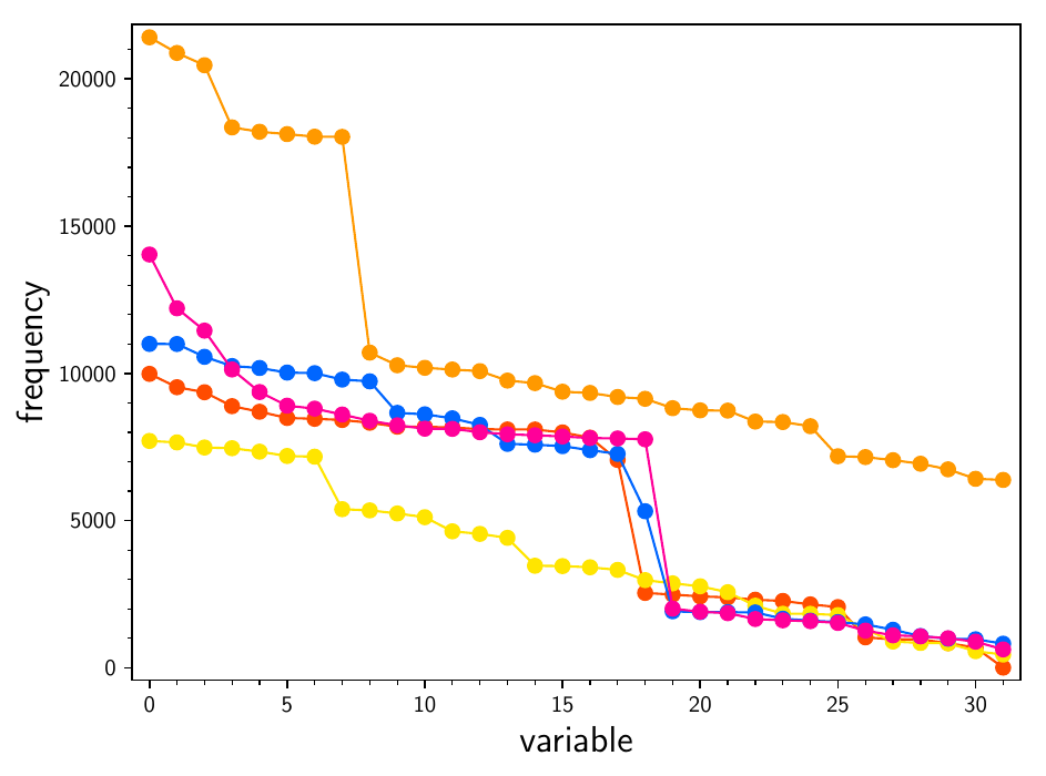
Figure rh. Frequencies of the key variables for five instances of \(\mathrm{SR}(2, 4, 2, 4)\)SR(2, 4, 2, 4). The variables are ordered according to their frequency.
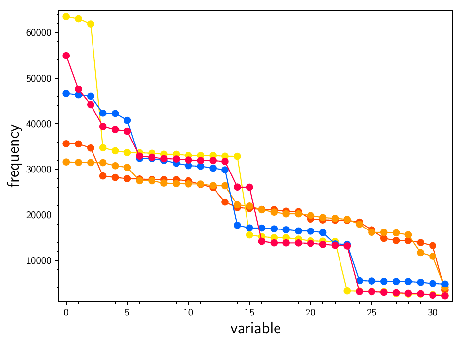
Table r7. Experiments with reduced polynomial systems and guessed variables. PT is the preprocessing time required to obtain the system.
| Cipher | Key bits | PT | F4 Time | F4 Mem. | SAT Time |
|---|---|---|---|---|---|
| SR(3, 2, 2, 4) | 16 | 8 min | 6 s | 33 MB | 35 s |
| SR(2, 4, 2, 4) | 32 | 2.5 min | 43 s | 620 MB | 9 min |
| SR(2, 2, 4, 4) | 32 | 31 s | 14 s | 72 MB | 5.5 min |
Epilogue
We demonstrated the capabilities of solving systems of polynomial equations by means of Gröbner bases and a SAT solver. Initially, we generated systems that contain auxiliary variables, and we saw that the SAT solver significantly outperformed Gröbner bases. We subsequently eliminated the auxiliary variables by a gradual substitution so that the systems contained only the variables of the initial secret key. The results were even worse compared to the systems with auxiliary variables. However, when we combined at least two systems with no auxiliary variables, we obtained much better results, especially for Gröbner bases — we were able to recover the secret key for one round of AES-128. We also solved one round of all the other ciphers with a reduced state array.
We showed that a 16-bit version of AES reaches its full diffusion after its third round. The polynomial system in the third round has the same properties as the system in the tenth round. From an algebraic cryptanalysis point of view, this might suggest that the original AES has enough spare rounds as well.
We tried reducing the polynomial systems without auxiliary variables by adding similar polynomials so that equal monomials would cancel each other out, and we also tried guessing the most frequent variables. The combination of these two approaches allowed us to obtain solutions for some of the systems that we could not solve otherwise.