AES as a System of Equations

AES (and its small scale derivatives) is a symmetric block cipher where the block is represented by the state, which is further divided into sub-blocks. AES is also an example of an iterated substitution-permutation network where one iteration is split into three stages (Shannon 1949). The first stage is a local nonlinear transformation (substitution) of the sub-blocks of the state. This transformation is performed by the SubBytes operation — the S-box is locally applied to each sub-block in order to substitute its value, while the mutual positions of the sub-blocks are left intact. This stage provides so-called confusion. The next stage is a global linear transformation of the state. This is performed by the ShiftRows and MixColumns operations, which are linear transformations over \(\mathrm{GF}(2^e)\), and which also change the mutual positions of the sub-blocks. This stage provides so-called diffusion, which tries to distribute the output bits of the S-boxes in the current iteration to as many S-box inputs as possible in the next iteration. The last stage is the addition of the key.

We now model AES and its scaled-down variants as a system of multivariate polynomial equations over \(\mathrm{GF}(2)\). We focus mainly on \(\mathrm{SR}(n, 2, 2, 4)\) and derive a system of equations for this cipher. A solution to this system provides the encryption key. Other scaled-down derivatives can be modeled in the same way, including AES itself. We use one ciphertext with its corresponding plaintext for our model. Our method therefore comes under the known-plaintext type of cryptanalysis.

Non-linear Equations

Consider the inversion part of the S-box. We have \(bc = 1\), where \(b \in \mathrm{GF}(2^e)\) is the input and \(c \in \mathrm{GF}(2^e)\) is the output of the S-box. This equation holds unless \(b = 0\), in which case we have \(b = c = 0\) and we say that a 0-inversion has taken place. The probability of a 0-inversion occurring is \(\frac{1}{16}\) when \(e = 4\) and \(\frac{1}{256}\) when \(e = 8\), so the probability of no 0-inversion occurring is \(\frac{15}{16}\) and \(\frac{255}{256}\), respectively. However, these probabilities hold for a single application of the S-box. In \(\mathrm{SR}(n, 2, 2, 4)\), there are four applications of the S-box per round during encryption, so the probability of no 0-inversions occurring during encryption is \((15/16)^{4n}\). There are also two applications of the S-box per round during the key schedule, so the probability of no 0-inversions occurring during the key schedule is \((15/16)^{2n}\). We presume statistical independence of the 0-inversions.

The actual occurrence of a 0-inversion during encryption or key schedule is deterministically given by the choice of the plaintext and initial key. If a 0-inversion occurs during the generation of the ciphertext, we can disregard the current combination of plaintext and key and pick another one. The issue, as we shall see, is that one of the equations modeling the S-box would have to change, and we as the cryptanalyst would not know which one since we do not know the key. For this reason, we assume that no 0-inversions have occurred for the given plaintext/key combination when we start generating the equations.

We regard both \(b = \sum_{i=0}^{3} b_i x^i\) and \(c = \sum_{i=0}^{3} c_i x^i\) as polynomials in \(\mathrm{GF}(2)[x]\). The product \(bc\) modulo the irreducible polynomial \(m(x) = x^4 + x + 1\) is \(r(x) = r_3 x^3 + r_2 x^2 + r_1 x + r_0\) where

\[\begin{aligned} r_0 &= b_0 c_0 \oplus b_3 c_1 \oplus b_2 c_2 \oplus b_1 c_3, \\ r_1 &= b_1 c_0 \oplus b_0 c_1 \oplus b_3 c_2 \oplus b_2 c_3 \oplus b_3 c_1 \oplus b_2 c_2 \oplus b_1 c_3, \\ r_2 &= b_2 c_0 \oplus b_1 c_1 \oplus b_0 c_2 \oplus b_3 c_3 \oplus b_3 c_2 \oplus b_2 c_3, \\ r_3 &= b_3 c_0 \oplus b_2 c_1 \oplus b_1 c_2 \oplus b_0 c_3 \oplus b_3 c_3. \end{aligned} \tag{ro}\]

Note that unlike in Remark rg, the coefficients \(b_i\) and \(c_i\) here are elements of \(\mathrm{GF}(2)\), not \(\mathrm{GF}(2^8)\), and the reduction is modulo \(x^4 + x + 1\) rather than \(x^4 + 1\). We have \(bc = r = 1\). This gives four multivariate quadratic equations over \(\mathrm{GF}(2)\): \(r_0 = 1\) and \(r_i = 0\) for \(i = 1, 2, 3\). These equations are bilinear in the \(b_i\) and \(c_i\) variables. For \(e = 8\), we would obtain eight multivariate quadratic equations instead of four.

If a 0-inversion occurred, the first equation would change to \(r_0 = 0\). However as already mentioned, we do not consider this case since we can detect 0-inversions before generating the equations and disregard the plaintext/key combinations that produce them.

Along with these equations, it is possible to obtain further quadratic equations from the relation \(bc = 1\). Notice that we also have \(bc^2 = c\) and \(b^2 c = b\). Let us focus on the first relation. The equations for \(b^2 c = b\) can be produced in the same fashion. Since we work over \(\mathrm{GF}(2)\), we can write \(bc^2 + c = 0\). Rather than multiplying the already-computed \(bc\) by \(c\) — which would introduce unnecessary intermediate cubic terms — we can compute the square of \(c\) and pre-multiply it by \(b\). Since we work over a commutative structure, the order of multiplication is irrelevant. To compute \(c^2\), we use equation ro and substitute \(c\) for \(b\). We obtain the polynomial \(d = c^2\) where \(d(x) = d_3 x^3 + d_2 x^2 + d_1 x + d_0\) with \[\begin{aligned} d_0 &= c_0 \oplus c_2, \\ d_1 &= c_2, \\ d_2 &= c_1 \oplus c_3, \\ d_3 &= c_3. \end{aligned}\] We can now obtain the final result \(t = bd + c\) where \(t(x) = t_3 x^3 + t_2 x^2 + t_1 x + t_0\) with \[\begin{aligned} t_0 &= b_0 c_0 \oplus b_0 c_2 \oplus b_3 c_2 \oplus b_2 c_1 \oplus b_2 c_3 \oplus b_1 c_3 \oplus c_0, \\ t_1 &= b_1 c_0 \oplus b_1 c_2 \oplus b_0 c_2 \oplus b_3 c_1 \oplus b_3 c_3 \oplus b_3 c_2 \oplus b_2 c_1 \oplus b_1 c_3 \oplus c_1, \\ t_2 &= b_2 c_0 \oplus b_2 c_2 \oplus b_1 c_2 \oplus b_0 c_1 \oplus b_0 c_3 \oplus b_3 c_1 \oplus b_2 c_3 \oplus c_2, \\ t_3 &= b_3 c_0 \oplus b_3 c_2 \oplus b_2 c_2 \oplus b_1 c_1 \oplus b_1 c_3 \oplus b_0 c_3 \oplus b_3 c_3 \oplus c_3. \end{aligned}\] We have \(t = 0\), so we obtain four equations \(t_i = 0\) for \(0 \le i < 4\). These equations are quadratic. We can obtain reciprocal equations from \(b^2 c = b\). All eight of these equations are biaffine in the \(b_i\) and \(c_i\) variables.

It is possible to obtain even more quadratic equations by considering the relations \(bc^4 = c^3\) and \(b^4 c = b^3\). Let us focus on the first one and rewrite it as \(bc^4 + c^3 = 0\). We can square \(d\) to obtain \(c^4\), so let \(f = d^2\) where \(f(x) = f_3 x^3 + f_2 x^2 + f_1 x + f_0\) with \[\begin{aligned} f_0 &= c_0 \oplus c_1 \oplus c_2 \oplus c_3, \\ f_1 &= c_1 \oplus c_3, \\ f_2 &= c_2 \oplus c_3, \\ f_3 &= c_3. \end{aligned}\] The polynomial \(c^3\) can be obtained by multiplying \(d\) by \(c\). We get \(g = dc\) where \(g(x) = g_3 x^3 + g_2 x^2 + g_1 x + g_0\) with \[\begin{aligned} g_0 &= c_0 \oplus c_0 c_2 \oplus c_1 c_2 \oplus c_1 c_3, \\ g_1 &= c_3 \oplus c_0 c_1 \oplus c_0 c_2 \oplus c_2 c_3, \\ g_2 &= c_2 \oplus c_0 c_1 \oplus c_0 c_2 \oplus c_0 c_3 \oplus c_1 c_2 \oplus c_1 c_3 \oplus c_2 c_3, \\ g_3 &= c_1 \oplus c_2 \oplus c_3 \oplus c_1 c_3 \oplus c_2 c_3. \end{aligned}\] We are now in a position to obtain the result \(u = bf + g\) where \(u(x) = u_3 x^3 + u_2 x^2 + u_1 x + u_0\) with \[\begin{aligned} u_0 &= b_3 c_3 \oplus b_3 c_1 \oplus b_2 c_3 \oplus b_2 c_2 \oplus b_1 c_3 \oplus b_0 c_3 \oplus b_0 c_2 \oplus b_0 c_1 \\ &\quad \oplus b_0 c_0 \oplus c_1 c_3 \oplus c_1 c_2 \oplus c_0 c_2 \oplus c_0, \\ u_1 &= b_3 c_2 \oplus b_3 c_1 \oplus b_2 c_2 \oplus b_1 c_2 \oplus b_1 c_1 \oplus b_1 c_0 \oplus b_0 c_3 \oplus b_0 c_1 \\ &\quad \oplus c_2 c_3 \oplus c_0 c_2 \oplus c_0 c_1 \oplus c_3, \\ u_2 &= b_3 c_2 \oplus b_2 c_2 \oplus b_2 c_1 \oplus b_2 c_0 \oplus b_1 c_3 \oplus b_1 c_1 \oplus b_0 c_3 \oplus b_0 c_2 \\ &\quad \oplus c_2 c_3 \oplus c_1 c_3 \oplus c_0 c_3 \oplus c_1 c_2 \oplus c_0 c_2 \oplus c_0 c_1 \oplus c_2, \\ u_3 &= b_3 c_2 \oplus b_3 c_1 \oplus b_3 c_0 \oplus b_2 c_3 \oplus b_2 c_1 \oplus b_1 c_3 \oplus b_1 c_2 \oplus b_0 c_3 \\ &\quad \oplus c_2 c_3 \oplus c_1 c_3 \oplus c_3 \oplus c_2 \oplus c_1. \end{aligned}\] We have \(u = 0\), so we obtain another four equations \(u_i = 0\) for \(0 \le i < 4\). These equations are still quadratic. We can obtain reciprocal equations from \(b^4 c = b^3\).

So far, we have derived 20 multivariate quadratic equations from the relation \(bc = 1\). A natural question arises whether we have identified all quadratic equations in the \(b_i\) and \(c_i\) variables. Notice, for example, that we have skipped the relation \(bc^3 = c^2\). The reason is that it would produce equations with cubic terms. Relations involving higher powers than \(c^4\) would also lead to equations with higher than quadratic terms. In fact, the 20 equations we have derived are all the quadratic equations over \(\mathrm{GF}(2)\). A further discussion can be found in (Cid, Murphy, and Robshaw 2006, 77). As also advised there, we focus on the first 12 bilinear and biaffine quadratic equations and omit the remaining eight. For \(e = 8\), we would obtain 40 multivariate quadratic equations instead of 20.

Linear Equations

The equations derived for the inversion part of the S-box account for the only non-linear equations in the whole system that models the \(\mathrm{SR}(n, 2, 2, 4)\) cipher. Let us now derive the remaining linear equations.

The affine transformation of the S-box can be expressed directly by equation rc where the input is the polynomial \(c(x)\) from the previous section. This gives four linear equations in the \(c_i\) variables. These equations together with the non-linear equations from the previous section fully describe a single S-box. Let \(L_s\) denote the matrix from equation rc. In order to describe the whole SubBytes operation, we extend the matrix \(L_s\) to the whole state array of \(\mathrm{SR}(n, 2, 2, 4)\): \[L = \begin{pmatrix} L_s & 0 & 0 & 0 \\ 0 & L_s & 0 & 0 \\ 0 & 0 & L_s & 0 \\ 0 & 0 & 0 & L_s \end{pmatrix}.\] We also extend the S-box constant vector \((0, 1, 1, 0)^T = 6_{16}\) to the vector \(\mathbf{6} = (6_{16}, 6_{16}, 6_{16}, 6_{16})\), covering the whole state array. We use \(\mathbf{b}\) to denote the input vector of the SubBytes operation and \(\mathbf{b^{-1}}\) to denote its output — the vector of the inverted elements in \(\mathrm{GF}(2^4)\). Each component in these vectors consists of the four coefficients of the polynomials \(b(x)\) and \(c(x)\), respectively, so we have 12 non-linear equations for each component.

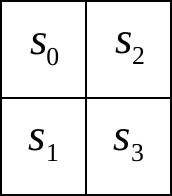
The actual state array is depicted in Figure rt. We represent it as the vector \((s_0, s_1, s_2, s_3)^T\). The ShiftRows operation can then be described by the matrix \[R = \begin{pmatrix} I_4 & 0 & 0 & 0 \\ 0 & 0 & 0 & I_4 \\ 0 & 0 & I_4 & 0 \\ 0 & I_4 & 0 & 0 \end{pmatrix}\] where \(I_4\) is the identity matrix of size four. Before describing the MixColumns operation, let us rewrite equation ro into matrix form:

\[\begin{pmatrix} r_0 \\ r_1 \\ r_2 \\ r_3 \end{pmatrix} = \begin{pmatrix} b_0 & b_3 & b_2 & b_1 \\ b_1 & b_0 \oplus b_3 & b_3 \oplus b_2 & b_2 \oplus b_1 \\ b_2 & b_1 & b_0 \oplus b_3 & b_3 \oplus b_2 \\ b_3 & b_2 & b_1 & b_0 \oplus b_3 \end{pmatrix} \begin{pmatrix} c_0 \\ c_1 \\ c_2 \\ c_3 \end{pmatrix}. \tag{r1}\]

If we substitute the binary values of the coefficients of the polynomials \(x + 1\) and \(x\) into equation r1, we get \[M_{x+1} = \begin{pmatrix} 1 & 0 & 0 & 1 \\ 1 & 1 & 0 & 1 \\ 0 & 1 & 1 & 0 \\ 0 & 0 & 1 & 1 \end{pmatrix} \qquad \text{and} \qquad M_x = \begin{pmatrix} 0 & 0 & 0 & 1 \\ 1 & 0 & 0 & 1 \\ 0 & 1 & 0 & 0 \\ 0 & 0 & 1 & 0 \end{pmatrix}.\] These matrices represent the multiplication by the polynomials \(x + 1\) and \(x\) modulo \(x^4 + x + 1\). The MixColumns operation, defined by equation rq, can then be expressed by the matrix \[M = \begin{pmatrix} M_{x+1} & M_x & 0 & 0 \\ M_x & M_{x+1} & 0 & 0 \\ 0 & 0 & M_{x+1} & M_x \\ 0 & 0 & M_x & M_{x+1} \end{pmatrix}.\] We can now describe one round of \(\mathrm{SR}(n, 2, 2, 4)\) by the expression

\[\mathbf{b_i} = MR(L \mathbf{b_{i-1}^{-1}} + \mathbf{6}) + \mathbf{k_i} \quad \text{for} \quad 1 \le i \le n \tag{ru}\] where \(\mathbf{k_i}\) is a vector containing 16 binary variables of the round key described in the following section and \(i\) is the round number. The vector \(\mathbf{b_{i-1}^{-1}}\) contains four components — the outputs from the S-boxes — each of which has four binary variables. It is straightforward to verify that \(R \mathbf{6} = M \mathbf{6} = \mathbf{6}\). We can then write \[\mathbf{b_i} = MRL \mathbf{b_{i-1}^{-1}} + \mathbf{k_i} + \mathbf{6} \quad \text{for} \quad 1 \le i \le n.\] This relation gives 16 linear equations representing one round of \(\mathrm{SR}(n, 2, 2, 4)\). In addition, we have 12 non-linear equations for each component in \(\mathbf{b_{i-1}^{-1}}\), so in total, we have \(16 + 4 \cdot 12 = 64\) equations describing one round of encryption. When \(i = n\), we have \[\mathbf{c_t} = MRL \mathbf{b_{n-1}^{-1}} + \mathbf{k_n} + \mathbf{6}\] where \(\mathbf{c_t}\) is the known ciphertext, a vector of 16 binary values. We obtain \(\mathbf{b_0}\) by adding the initial unknown key \(\mathbf{k_0}\) to the known plaintext \(\mathbf{p_t}\): \[\mathbf{b_0} = \mathbf{p_t} + \mathbf{k_0}.\] This addition gives 16 initial equations where \(\mathbf{p_t}\) is a vector of 16 binary values and \(\mathbf{k_0}\) is a vector of 16 binary variables. Our goal is to compute the values of \(\mathbf{k_0}\) since this is the user’s key. All other variables are auxiliary.

Key Schedule Equations

The generation of round keys for \(\mathrm{SR}(n, r, c, e)\) is thoroughly described in (Cid, Murphy, and Robshaw 2005). Let us describe the equations for \(\mathrm{SR}(n, 2, 2, 4)\). Let \(\mathbf{k_i} = (k_{i,0}, k_{i,1}, k_{i,2}, k_{i,3})^T \in \mathrm{GF}(2^4)^4\) be the round key of round \(i\). The round key can then be defined by \[\begin{pmatrix} k_{i,2q} \\ k_{i,2q+1} \end{pmatrix} = \begin{pmatrix} L k_{i-1,3}^{-1} \\ L k_{i-1,2}^{-1} \end{pmatrix} + \begin{pmatrix} 6_{16} \\ 6_{16} \end{pmatrix} + \begin{pmatrix} x^{i-1} \\ 0 \end{pmatrix} + \sum_{t=0}^{q} \begin{pmatrix} k_{i-1,2t} \\ k_{i-1,2t+1} \end{pmatrix}\] for \(0 \le q < 2\) where \(x^{i-1}\) is an element of \(\mathrm{GF}(2^4)\). This expression gives 16 linear equations for each \(\mathbf{k_i}\). The initial key \(\mathbf{k_0}\) is not provided by the user — it is a vector of 16 binary variables that we, as the cryptanalyst, are trying to compute. We also get \(2 \cdot 12 = 24\) non-linear equations since the computation of each \(\mathbf{k_i}\) requires two applications of the S-box. One round of the key schedule in \(\mathrm{SR}(n, 2, 2, 4)\) is then described by 40 equations.

Equations without Auxiliary Variables

We can also derive equations that contain only the variables of the initial key. To obtain such a system, we eliminate the auxiliary variables by a gradual substitution of the initial key variables since we know that the cipher starts by adding the initial key to the known plaintext. It is straightforward to perform this substitution for the linear equations. For the non-linear equations modeling the S-box, we can leverage Gröbner bases. Consider the four polynomials \(r_0, \ldots, r_3\) from equation ro as polynomials in \(\mathbb{F}[c_0, \ldots, c_3, b_0, \ldots, b_3]\). It is not straightforward to express the output bits \(c_i\) in terms of the input bits \(b_i\) by ordinary manipulation techniques. If we impose a block order \(\succeq_{\mathrm{grlex}, \mathrm{grlex}}\) on \(\mathbb{F}[c_0, \ldots, c_3, b_0, \ldots, b_3]\) with \(\succeq_{\mathrm{grlex}}\) on both \(\mathbb{F}[c_0, \ldots, c_3]\) and \(\mathbb{F}[b_0, \ldots, b_3]\), and compute the reduced Gröbner basis, we get the following polynomial system:

\[\begin{aligned} f_1 &= c_0 \oplus b_2 b_1 b_0 \oplus b_3 b_2 b_1 \oplus b_2 b_0 \oplus b_2 b_1 \oplus b_0 \oplus b_1 \oplus b_2 \oplus b_3, \\ f_2 &= c_1 \oplus b_3 b_1 b_0 \oplus b_1 b_0 \oplus b_2 b_0 \oplus b_2 b_1 \oplus b_3 b_1 \oplus b_3, \\ f_3 &= c_2 \oplus b_3 b_2 b_0 \oplus b_1 b_0 \oplus b_2 b_0 \oplus b_3 b_0 \oplus b_2 \oplus b_3, \\ f_4 &= c_3 \oplus b_3 b_2 b_1 \oplus b_3 b_0 \oplus b_3 b_1 \oplus b_3 b_2 \oplus b_1 \oplus b_2 \oplus b_3, \\ f_5 &= b_3 b_2 b_1 b_0 \oplus b_2 b_1 b_0 \oplus b_3 b_1 b_0 \oplus b_3 b_2 b_0 \oplus b_3 b_2 b_1 \oplus b_1 b_0 \oplus b_2 b_0 \\ &\quad \oplus b_2 b_1 \oplus b_3 b_0 \oplus b_3 b_1 \oplus b_3 b_2 \oplus b_0 \oplus b_1 \oplus b_2 \oplus b_3 \oplus 1. \end{aligned} \tag{rw}\]

The last polynomial \(f_5\) involves only the variables \(b_i\). This polynomial is not satisfied only when all \(b_i = 0\) and it holds whenever at least one \(b_i = 1\). Since we do not consider 0-inversions, this polynomial is always satisfied and we can omit it from the system. In the remaining polynomials, the output variables \(c_0, \ldots, c_3\) are expressed solely in terms of the input variables \(b_i\). This allows us to perform the gradual substitution of the unknown variables of the initial key \(\mathbf{k_0}\) throughout the whole polynomial system. After the substitution, we obtain \(|\mathbf{k_0}| = 16\) polynomials. The size of these polynomials is close to \(2^{|\mathbf{k_0}| - 1}\) at full diffusion of the cipher. The diffusion grows rapidly with each round. For example, the cipher \(\mathrm{SR}(n, 2, 2, 4)\) reaches its full diffusion at round \(n = 3\). This way of generating the polynomials is therefore suitable only for low values of \(n\). A different method for obtaining polynomials without auxiliary variables is described in (Bulygin and Brickenstein 2010).

Yet another way of obtaining polynomials involving only the variables of the initial key \(\mathbf{k_0}\) is to regard the cipher as a set of boolean functions of \(\mathbf{k_0}\), one function per bit of \(\mathbf{k_0}\). We can then convert such functions into an Algebraic Normal Form (ANF) in order to obtain the polynomials. Such a conversion can be found in (Saarinen 2006). However, the complexity of this approach requires at least \(|\mathbf{k_0}| \cdot 2^{|\mathbf{k_0}|}\) encryptions even if we consider only one round of the cipher. For this reason, we do not examine this method further.

References